# install packages
# install.packages("dplyr")
# install.packages("matrixcalc")
# install.packages("earth")

library(dplyr)
library(matrixcalc)
library(earth)Regression Calibration Demo
In this demo, we mainly focus on correcting for measurement error in covariates when the outcome is binary.
1. Two Methods for Regression Calibration if Validation Study Available
Imputation Method (RC-IM): regCalibCRS
Deattenuation Factor Method (RC-DF): regCalibRSW
1.1 Introduction to Data Set
The data is from a Study on Dietary Fat Intake and the Risk of Breast Cancer
Main Study: 89,538 women returned a food frequency questionnaire (FFQ) in 1980 in the Nurses’ Health Study (NHS).
Breast cancer incidence over the first 4 years of the follow-up was ascertained by self-report and validated through medical records review.
Dietary intake (Z) was measured through a 61-item FFQ asking about the usual frequency of intake of the most common foods during the past year.
Validation Study: 173 women from the MS.
- The VS participants recorded 4 one-week diet records (X) based on weighed food intake at 3-month intervals over a one-year period in 1981.
Variable Dictionary
fq*: Questionnaire-based error-prone surrogates.
dr*: diet-record-based (more accurate) dietary intakes derived from the 4 one-week diet records in the validation study.
Variables contained in both main and validation data:
fqcal: Daily total caloric intake obtained from the dietary questionnaire (kcal/day).
fqcalinc: Daily total caloric intake from the dietary questionnaire, expressed in units of 800 kcal/day.
fqtfat: Daily total fat intake obtained from the dietary questionnaire (g/day).
fqtfatinc: Daily total fat intake from the dietary questionnaire, expressed in units of 10 g/day.
fqalc: Daily alcohol intake obtained from the dietary questionnaire (g/day).
fqalcinc: Daily alcohol intake from the dietary questionnaire, expressed in units of 12 g/day.
age: Age in years
agec: Discretized age: <40, [40, 45), [45, 55), [50,55),>=50
Variables contained in main data:
- case: Binary outcome variable, if the breast cancer occurred during the four year follow-up
Contained in validation data:
drcal: Daily total caloric intake from the diet record (kcal/day).
drcalinc: Daily total caloric intake from the diet record, expressed in units of 800 kcal/day.
drtfat: Daily total fat intake from the diet record (g/day).
drtfatinc: Daily total fat intake from the diet record, expressed in units of 10 g/day.
dralc: Daily alcohol intake from the diet record (g/day).
dralcinc: Daily alcohol intake from the diet record, expressed in units of 12 g/day.
1.2 Importing Data
Data Use Notice: The dataset provided here is for educational use in this short course only and can not be copied, redistributed, or used for any other purpose.
# read in the main study data
main_data<-read.csv("main_data_external.csv",row.names = 1)

# read in the validation study data
valid_data<-read.csv("valid_data_external.csv",row.names = 1)

# show the first 5 rows of the data
head(main_data)
id fqcal fqcalinc fqtfat fqtfatinc fqalc fqalcinc age agec case
1 100008 1661 2.07625 88 8.8 8.413 0.7010833 48.75000 45~50 0
2 100013 1573 1.96625 65 6.5 0.000 0.0000000 37.83333 <40 0
3 100015 1071 1.33875 44 4.4 7.549 0.6290833 45.66667 45~50 0
4 100017 1000 1.25000 52 5.2 29.114 2.4261667 48.08333 45~50 0
5 100018 2013 2.51625 79 7.9 11.137 0.9280833 54.91667 50~55 0
6 100022 3073 3.84125 133 13.3 0.000 0.0000000 52.50000 50~55 0head(valid_data) id fqcal fqcalinc fqtfat fqtfatinc fqalc fqalcinc drcal drcalinc drtfat
1 100396 1242.2 1.552750 53.8 5.38 1.68 0.1400000 1807 2.25875 81.15
2 100566 907.0 1.133750 36.6 3.66 0.00 0.0000000 1418 1.77250 53.28
3 107633 786.0 0.982500 47.2 4.72 15.10 1.2583333 1889 2.36125 83.48
4 107737 1392.5 1.740625 55.3 5.53 7.49 0.6241667 1426 1.78250 49.65
5 107744 1259.8 1.574750 71.0 7.10 12.84 1.0700000 1253 1.56625 55.18
6 107813 987.1 1.233875 41.1 4.11 0.00 0.0000000 1699 2.12375 73.83
drtfatinc dralc dralcinc age agec
1 8.115 8.26 0.68833333 39 <40
2 5.328 0.83 0.06916667 49 45~50
3 8.348 20.13 1.67750000 43 40~45
4 4.965 11.16 0.93000000 51 50~55
5 5.518 7.18 0.59833333 53 50~55
6 7.383 1.76 0.14666667 54 50~551.3 Data Exploration
Comparing the mean and standard deviation of questionnaire-based measures and diet record-based record measures in the validation study.
summary_table1<-matrix(NA, nrow = 3, ncol=4)
summary_table1[1,]<-c(mean(valid_data$fqcal), sd(valid_data$fqcal), mean(valid_data$drcal), sd(valid_data$drcal))
summary_table1[2,]<-c(mean(valid_data$fqtfat), sd(valid_data$fqtfat), mean(valid_data$drtfat), sd(valid_data$drtfat))
summary_table1[3,]<-c(mean(valid_data$fqalc), sd(valid_data$fqalc), mean(valid_data$dralc), sd(valid_data$dralc))
row.names(summary_table1)<-c("Total calories", "Total fat", "Alcohol intakes")
colnames(summary_table1)<-c("Mean (fq)", "SD (fq)", "Mean (dr)", "SD (dr)")
round(summary_table1,2)
Mean (fq) SD (fq) Mean (dr) SD (dr)
Total calories 1371.73 482.05 1619.87 323.41
Total fat 56.08 21.97 68.62 16.29
Alcohol intakes 8.95 12.25 8.96 9.66Correlation between questionnaire-based measure and diet record-based record measures in the validation study.
Summary_table2<-cor(valid_data[, c(2,4,6)], valid_data[,c(8,10,12)])
Summary_table2
drcal drtfat dralc
fqcal 0.3559695 0.2987738 -0.06172778
fqtfat 0.3150312 0.3696641 0.01036997
fqalc 0.1974423 0.1308419 0.84988383The measures of total calories, total fat, and alcohol intakes from questionnaire and diet records are correlated.
cor(valid_data[, c(2,4,6)]) fqcal fqtfat fqalc
fqcal 1.0000000000 0.88621802 -0.0005010716
fqtfat 0.8862180190 1.00000000 0.0760384810
fqalc -0.0005010716 0.07603848 1.0000000000cor(valid_data[,c(8,10,12)]) drcal drtfat dralc
drcal 1.0000000 0.88453882 0.20152169
drtfat 0.8845388 1.00000000 0.09584735
dralc 0.2015217 0.09584735 1.00000000Outcome model: \[ \begin{aligned} &logit(\text{Probability of breast cancer occured})\\ &\sim\text{fat }(10g/day)\;+\;\text{calories }(800kcal/day)\;+\;\text{alcohol }(12g/day)\\ &\quad +\; \mathbf{1}\!\left(\text{age}\in[40,45)\right) +\mathbf{1}\!\left(\text{age}\in[45,50)\right) +\mathbf{1}\!\left(\text{age}\in[50,55)\right) +\mathbf{1}\!\left(\text{age}\ge 50\right). \end{aligned} \]
(age \(<40\) is the reference category for age.)
1.4 Naive Analysis
# Logistic regression in the MS

uncorrected <- glm(case ~ fqtfatinc + fqcalinc + fqalcinc + agec, data=main_data, family=binomial(link = "logit"))
# calculating the OR and CI
uncorrected_results<-exp(cbind(OR = coef(uncorrected), confint(uncorrected)))
uncorrected_results
OR 2.5 % 97.5 %
(Intercept) 0.00380417 0.002696806 0.00531978
fqtfatinc 0.97883434 0.924601002 1.03613092
fqcalinc 1.00207749 0.770922385 1.29395543
fqalcinc 1.14859818 1.064814610 1.23386158
agec>=50 2.66079494 2.004133696 3.56370240
agec40~45 1.41923883 1.041903968 1.94118652
agec45~50 2.28648649 1.731062686 3.04929876
agec50~55 2.25490565 1.702950573 3.013373601.5 Regression Calibration – Deattenuation Factor Method (RC-DF)
Assumptions
Surrogacy
Transportability
Logistic-linearity of the outcome model
Linearity in the measurement error model
\[ \begin{aligned} \mathrm{DR\_Alcohol}(12g/day) &\sim\mathrm{FFQ\_Alcohol}(12g/day) + \mathrm{FFQ\_Total\_Fat}(10g/day) + \mathrm{FFQ\_Calories}(800kcal/day) \\ &\quad + \mathbf{1}\!\left(\mathrm{Age}\in[40,45)\right) + \mathbf{1}\!\left(\mathrm{Age}\in[45,50)\right) + \mathbf{1}\!\left(\mathrm{Age}\in[50,55)\right) + \mathbf{1}\!\left(\mathrm{Age}\ge 50\right), \\[6pt] \mathrm{DR\_Total\_Fat}(10g/day) &\sim \mathrm{FFQ\_Total\_Fat}(10g/day) + \mathrm{FFQ\_Alcohol}(12g/day) + \mathrm{FFQ\_Calories}(800kcal/day) \\ &\quad + \mathbf{1}\!\left(\mathrm{Age}\in[40,45)\right) + \mathbf{1}\!\left(\mathrm{Age}\in[45,50)\right) + \mathbf{1}\!\left(\mathrm{Age}\in[50,55)\right) + \mathbf{1}\!\left(\mathrm{Age}\ge 50\right), \\[6pt] \mathrm{DR\_Calories}(800kcal/day) &\sim \mathrm{FFQ\_Calories}(800kcal/day) + \mathrm{FFQ\_Alcohol}(12g/day) + \mathrm{FFQ\_Total\_Fat}(10g/day) \\ &\quad + \mathbf{1}\!\left(\mathrm{Age}\in[40,45)\right) + \mathbf{1}\!\left(\mathrm{Age}\in[45,50)\right) + \mathbf{1}\!\left(\mathrm{Age}\in[50,55)\right) + \mathbf{1}\!\left(\mathrm{Age}\ge 50\right). \end{aligned} \]
For logistic regression, at least one of the following two conditions should hold:
Small measurement error variance
Rare disease outcome plus normally distributed homoscedastic error
Running code
source("regCalibRSW.R")rcdf <- regCalibRSW(supplyEstimates = FALSE,
ms = main_data,
vs = valid_data,
sur = c("fqtfatinc","fqcalinc","fqalcinc"), # mismeasured exposures and covaraites
exp = c("drtfatinc","drcalinc","dralcinc"),
covCalib = c("agec"),
covOutcome = NULL, # Correctly measured risk factors for outcome in the MS
# Should not include any variable from `covCalib`
outcome = "case",
method = "glm", # methods for outcome modeling
family = binomial, # family parameter being passed to glm
link = "logit", # link function being passed to glm
external = TRUE, # Indicates whether `vs` is an external validation set.
pointEstimates = NA,
vcovEstimates = NA
)#Corrected regression coefficients (exponentiated)
corrected_RC_DF<-exp(cbind(OR = rcdf$correctedCoefTable[,1],
'2.5 %' = rcdf$correctedCoefTable[,5],
'97.5 %' = rcdf$correctedCoefTable[,6]))# compare results from naive and RC-DF methods
cbind(uncorrected_results[-1,],corrected_RC_DF) OR 2.5 % 97.5 % OR 2.5 % 97.5 %
fqtfatinc 0.9788343 0.9246010 1.036131 0.9335793 0.7938682 1.097878
fqcalinc 1.0020775 0.7709224 1.293955 1.0069521 0.4517235 2.244631
fqalcinc 1.1485982 1.0648146 1.233862 1.2436176 1.0766925 1.436422
agec>=50 2.6607949 2.0041337 3.563702 2.5370281 1.8622682 3.456275
agec40~45 1.4192388 1.0419040 1.941187 1.4257748 1.0381491 1.958133
agec45~50 2.2864865 1.7310627 3.049299 2.1405215 1.5678133 2.922435
agec50~55 2.2549056 1.7029506 3.013374 2.1353751 1.5683911 2.9073281.6 Regression Calibration – Imputation Method (RC-IM)
Assumptions
- Surrogacy
- Transportability
- Logistic-linearity of the outcome model
- The measurement error model is not limited to linear
- For logistic regression, at least one of the following two conditions should hold:
Small measurement error variance
Rare disease outcome plus normally distributed homoscedastic error
Running code
- Assume the measurement error model is linear.
# source the function for RC-IM
source("regCalibCRS.R") echo=FALSE
# call regCalibCRS
rcim <- regCalibCRS(ms = main_data, #MS
vs = valid_data, #VS
sur = c("fqtfatinc","fqcalinc","fqalcinc"), #Mismeasured exposures and covaraites
exp = c("drtfatinc","drcalinc","dralcinc"),
#Correctly measured exposure and covaraites with one-to-one correspondence to `sur`
covCalib = c("agec"),
#Error-free covariates to adjust for in calibration model including non-linear terms.
covOutcome = c("agec"),
#Error-free covariates to adjust for in outcome model including non-linear terms.
outcome = "case",
method = "glm", #Methods for outcome modeling
family = binomial, #Family parameter being passed to glm
link = "logit", #Link function being passed to glm
external = TRUE #Indicates whether `vs` is an external validation set.
)#Corrected regression coefficients (exponentiated)
corrected_RC_IM<-exp(cbind(OR = rcim$correctedCoefTable[,1],
'2.5 %' = rcim$correctedCoefTable[,5],
'97.5 %' = rcim$correctedCoefTable[,6]))corrected_RC_IM OR 2.5 % 97.5 %
drtfatinc 0.9335793 0.7938254 1.097937
drcalinc 1.0069521 0.4353128 2.329251
dralcinc 1.2436176 1.0547162 1.466352
agec>=50 2.5370281 1.9089889 3.371686
agec40~45 1.4257748 1.1067126 1.836822
agec45~50 2.1405215 1.6312957 2.808707
agec50~55 2.1353751 1.6308090 2.796052Results Comparison
Compare the OR among naive, deattenuation factor, and imputation methods.
combine_results1<-as.data.frame(round(cbind(uncorrected_results[-1,], corrected_RC_DF, corrected_RC_IM),2))
combine_results1
OR 2.5 % 97.5 % OR 2.5 % 97.5 % OR 2.5 % 97.5 %
fqtfatinc 0.98 0.92 1.04 0.93 0.79 1.10 0.93 0.79 1.10
fqcalinc 1.00 0.77 1.29 1.01 0.45 2.24 1.01 0.44 2.33
fqalcinc 1.15 1.06 1.23 1.24 1.08 1.44 1.24 1.05 1.47
agec>=50 2.66 2.00 3.56 2.54 1.86 3.46 2.54 1.91 3.37
agec40~45 1.42 1.04 1.94 1.43 1.04 1.96 1.43 1.11 1.84
agec45~50 2.29 1.73 3.05 2.14 1.57 2.92 2.14 1.63 2.81
agec50~55 2.25 1.70 3.01 2.14 1.57 2.91 2.14 1.63 2.80Exercise: Assume that only total fat intake (fqtfatinc) is measured with error, whereas total calorie intake and alcohol intake (fqcalinc and fqalcinc) are measured without error. How should the code be modified for the two methods under this assumption? How do the resulting estimates compare with those obtained from the model in which all three exposures are treated as error-prone?
Hint
Use the following calibration model:
drtfatinc ~ fqtfatinc + fqcalinc + fqalcinc + agecUse the following outcome model:
Cas ~ drtfatinc + fqcalinc + fqalcinc + agec
Deattenuation factor method:
#Deattenuation factor method
rcdf_fat <- regCalibRSW(supplyEstimates = FALSE,
ms = main_data,
vs = valid_data,
sur = c("fqtfatinc"), # mismeasured exposures and covaraites
exp = c("drtfatinc"),
covCalib = c("fqcalinc","fqalcinc", "agec"),
covOutcome = NULL, # Correctly measured risk factors for outcome in the MS
# Should not include any variable from `covCalib`
outcome = "case",
method = "glm", # methods for outcome modeling
family = binomial, # family parameter being passed to glm
link = "logit", # link function being passed to glm
external = TRUE, # Indicates whether `vs` is an external validation set.
pointEstimates = NA,
vcovEstimates = NA
)

#Corrected regression coefficients (exponentiated)
corrected_RC_DF_fat<-exp(cbind(OR = rcdf_fat$correctedCoefTable[,1],
'2.5 %' = rcdf_fat$correctedCoefTable[,5],
'97.5 %' = rcdf_fat$correctedCoefTable[,6]))

# print results
corrected_RC_DF_fat
OR 2.5 % 97.5 %
drtfatinc 0.9341930 0.7744417 1.126898
fqcalinc 0.9831908 0.7888872 1.225352
fqalcinc 1.1582462 1.0759887 1.246792
agec>=50 2.5440034 1.8461166 3.505712
agec40~45 1.4126969 1.0320012 1.933828
agec45~50 2.1393680 1.5255212 3.000217
agec50~55 2.1398589 1.5469335 2.960047combine_results2<-as.data.frame(round(cbind(uncorrected_results[-1,], corrected_RC_DF, corrected_RC_DF_fat),2))
combine_results2 OR 2.5 % 97.5 % OR 2.5 % 97.5 % OR 2.5 % 97.5 %
fqtfatinc 0.98 0.92 1.04 0.93 0.79 1.10 0.93 0.77 1.13
fqcalinc 1.00 0.77 1.29 1.01 0.45 2.24 0.98 0.79 1.23
fqalcinc 1.15 1.06 1.23 1.24 1.08 1.44 1.16 1.08 1.25
agec>=50 2.66 2.00 3.56 2.54 1.86 3.46 2.54 1.85 3.51
agec40~45 1.42 1.04 1.94 1.43 1.04 1.96 1.41 1.03 1.93
agec45~50 2.29 1.73 3.05 2.14 1.57 2.92 2.14 1.53 3.00
agec50~55 2.25 1.70 3.01 2.14 1.57 2.91 2.14 1.55 2.96Imputation method:
# For Imputation method:
rcim_fat <- regCalibCRS(ms = main_data, #MS
vs = valid_data, #VS
sur = c("fqtfatinc"), #Mismeasured exposures and covaraites
exp = c("drtfatinc"),
#Correctly measured exposure and covaraites with one-to-one correspondence to `sur`
covCalib = c("fqcalinc","fqalcinc", "agec"),
#Error-free covariates to adjust for in calibration model including non-linear terms.
covOutcome = c("fqcalinc","fqalcinc", "agec"),
#Error-free covariates to adjust for in outcome model including non-linear terms.
outcome = "case",
method = "glm", #Methods for outcome modeling
family = binomial, #Family parameter being passed to glm
link = "logit", #Link function being passed to glm
external = TRUE #Indicates whether `vs` is an external validation set.
)corrected_RC_IM_fat<-exp(cbind(OR = rcim_fat$correctedCoefTable[,1],
'2.5 %' = rcim_fat$correctedCoefTable[,5],
'97.5 %' = rcim_fat$correctedCoefTable[,6]))
corrected_RC_IM_fat OR 2.5 % 97.5 %
drtfatinc 0.9341930 0.7698826 1.133571
fqcalinc 0.9831908 0.7811568 1.237478
fqalcinc 1.1582462 1.0581005 1.267870
agec>=50 2.5440034 1.8763931 3.449146
agec40~45 1.4126969 1.0991324 1.815716
agec45~50 2.1393680 1.5592900 2.935243
agec50~55 2.1398589 1.5907076 2.878591combine_results3<-as.data.frame(round(cbind(uncorrected_results[-1,], corrected_RC_IM, corrected_RC_IM_fat),2))
combine_results3 OR 2.5 % 97.5 % OR 2.5 % 97.5 % OR 2.5 % 97.5 %
fqtfatinc 0.98 0.92 1.04 0.93 0.79 1.10 0.93 0.77 1.13
fqcalinc 1.00 0.77 1.29 1.01 0.44 2.33 0.98 0.78 1.24
fqalcinc 1.15 1.06 1.23 1.24 1.05 1.47 1.16 1.06 1.27
agec>=50 2.66 2.00 3.56 2.54 1.91 3.37 2.54 1.88 3.45
agec40~45 1.42 1.04 1.94 1.43 1.11 1.84 1.41 1.10 1.82
agec45~50 2.29 1.73 3.05 2.14 1.63 2.81 2.14 1.56 2.94
agec50~55 2.25 1.70 3.01 2.14 1.63 2.80 2.14 1.59 2.881.7 Nonlinearity in the Measurement Error Model
In the VS, we will fit the following non-linear measurement error models: \[ \begin{aligned} \mathrm{DR\_Alcohol}(12g/day) &= \mathrm{FFQ\_Alcohol}(12g/day) + \mathrm{FFQ\_Total\_Fat}(10g/day) + \mathrm{FFQ\_Calories}(800kcal/day) \\ &\quad + \mathbf{1}\!\left(\mathrm{Age}\in[40,45)\right) + \mathbf{1}\!\left(\mathrm{Age}\in[45,50)\right) + \mathbf{1}\!\left(\mathrm{Age}\in[50,55)\right) + \mathbf{1}\!\left(\mathrm{Age}\ge 50\right)\\ &\quad +\text{Spline Terms for FFQ_Alcohol}, \\[6pt] \mathrm{DR\_Total\_Fat}(10g/day) &= \mathrm{FFQ\_Total\_Fat}(10g/day) + \mathrm{FFQ\_Alcohol}(12g/day) + \mathrm{FFQ\_Calories}(800kcal/day) \\ &\quad + \mathbf{1}\!\left(\mathrm{Age}\in[40,45)\right) + \mathbf{1}\!\left(\mathrm{Age}\in[45,50)\right) + \mathbf{1}\!\left(\mathrm{Age}\in[50,55)\right) + \mathbf{1}\!\left(\mathrm{Age}\ge 50\right)\\ &\quad +\text{Spline Terms for FFQ_Alcohol}, \\[6pt] \mathrm{DR\_Calories}(800kcal/day) &= \mathrm{FFQ\_Calories}(800kcal/day) + \mathrm{FFQ\_Alcohol}(12g/day) + \mathrm{FFQ\_Total\_Fat}(10g/day) \\ &\quad + \mathbf{1}\!\left(\mathrm{Age}\in[40,45)\right) + \mathbf{1}\!\left(\mathrm{Age}\in[45,50)\right) + \mathbf{1}\!\left(\mathrm{Age}\in[50,55)\right) + \mathbf{1}\!\left(\mathrm{Age}\ge 50\right)\\ &\quad +\text{Spline Terms for FFQ_Alcohol}. \end{aligned} \]
Violation of Measurement Error Model Linearity Assumption: Sensitivity Analysis using RC-IM
library(Hmisc)
# Data preparation - create spline terms for alcohol
rcsalcList <- paste0("rcsfqalc.", seq(1,3))
# Include spline terms for every 12 g/day increment in alcohol in both MS and VS
rcsfqalc.main <- rcspline.eval(main_data$fqalcinc, knots=c(0.5,1,1.5,2,4))
colnames(rcsfqalc.main) <- rcsalcList
main1 <- cbind(main_data, rcsfqalc.main) %>% as.data.frame()
rcsfqalc <- rcspline.eval(valid_data$fqalcinc, knots=c(0.5,1,1.5,2,4))
colnames(rcsfqalc) <- rcsalcList
valid1 <- cbind(valid_data, rcsfqalc) %>% as.data.frame()
rcim_nl <- regCalibCRS(ms = main1, # MS
vs = valid1, # VS
sur = c("fqtfatinc","fqcalinc","fqalcinc"),
exp = c("drtfatinc","drcalinc","dralcinc"),
covCalib = c("agec", "rcsfqalc.1", "rcsfqalc.2", "rcsfqalc.3"),
# error-free covariates to adjust for in calibration model
# spline terms adjusted in the ME models included here
covOutcome = c("agec"),
# error-free covariates to adjust for in outcome model
# including non-linear terms.
outcome = "case",
method = "glm", # methods for outcome modeling
family = binomial, # family parameter being passed to glm
link = "logit", # link function being passed to glm
external = TRUE # Indicates whether `vs` is an external validation set.
)# Print out results on OR scale
imputed_nl_results<-exp(cbind(OR = rcim_nl$correctedCoefTable[,1],
'2.5 %' = rcim_nl$correctedCoefTable[,5],
'97.5 %' = rcim_nl$correctedCoefTable[,6]))
imputed_nl_results OR 2.5 % 97.5 %
drtfatinc 0.9563098 0.8226921 1.111629
drcalinc 0.8926449 0.4134614 1.927181
dralcinc 1.2724962 1.1001239 1.471876
agec>=50 2.5185785 1.9113127 3.318786
agec40~45 1.4072803 1.0974011 1.804662
agec45~50 2.1403372 1.6423450 2.789331
agec50~55 2.1481155 1.6565357 2.785572Compare results from naive, deattenuation, imputed methods and imputed method with nonlinear measurement error model:
Comparison_df<-as.data.frame(round(cbind(uncorrected_results[-1,], corrected_RC_DF, corrected_RC_IM, imputed_nl_results),2))
Comparison_df
OR 2.5 % 97.5 % OR 2.5 % 97.5 % OR 2.5 % 97.5 % OR 2.5 %
fqtfatinc 0.98 0.92 1.04 0.93 0.79 1.10 0.93 0.79 1.10 0.96 0.82
fqcalinc 1.00 0.77 1.29 1.01 0.45 2.24 1.01 0.44 2.33 0.89 0.41
fqalcinc 1.15 1.06 1.23 1.24 1.08 1.44 1.24 1.05 1.47 1.27 1.10
agec>=50 2.66 2.00 3.56 2.54 1.86 3.46 2.54 1.91 3.37 2.52 1.91
agec40~45 1.42 1.04 1.94 1.43 1.04 1.96 1.43 1.11 1.84 1.41 1.10
agec45~50 2.29 1.73 3.05 2.14 1.57 2.92 2.14 1.63 2.81 2.14 1.64
agec50~55 2.25 1.70 3.01 2.14 1.57 2.91 2.14 1.63 2.80 2.15 1.66
97.5 %
fqtfatinc 1.11
fqcalinc 1.93
fqalcinc 1.47
agec>=50 3.32
agec40~45 1.80
agec45~50 2.79
agec50~55 2.79Exercise
If only total fat intake (fqtfatinc) is measured with error, whereas total calorie intake and alcohol intake (fqcalinc and fqalcinc) are measured accurately, how should the code for the imputation method be modified when the measurement error model is nonlinear in alcohol?
rcim_nl_fat <- regCalibCRS(ms = main1, # MS
vs = valid1, # VS
sur = c("fqtfatinc"),
exp = c("drtfatinc"),
covCalib = c("fqcalinc","fqalcinc", "agec", "rcsfqalc.1", "rcsfqalc.2", "rcsfqalc.3"),
# error-free covariates to adjust for in calibration model
# spline terms adjusted in the ME models included here
covOutcome = c("fqcalinc","fqalcinc", "agec"),
# error-free covariates to adjust for in outcome model
# including non-linear terms.
outcome = "case",
method = "glm", # methods for outcome modeling
family = binomial, # family parameter being passed to glm
link = "logit", # link function being passed to glm
external = TRUE # Indicates whether `vs` is an external validation set.
)
# Print out results on OR scale
imputed_nl_results<-exp(cbind(OR = rcim_nl$correctedCoefTable[,1],
'2.5 %' = rcim_nl$correctedCoefTable[,5],
'97.5 %' = rcim_nl$correctedCoefTable[,6]))
imputed_nl_results OR 2.5 % 97.5 %
drtfatinc 0.9563098 0.8226921 1.111629
drcalinc 0.8926449 0.4134614 1.927181
dralcinc 1.2724962 1.1001239 1.471876
agec>=50 2.5185785 1.9113127 3.318786
agec40~45 1.4072803 1.0974011 1.804662
agec45~50 2.1403372 1.6423450 2.789331
agec50~55 2.1481155 1.6565357 2.785572Testing the linearity of the measurement error model
#install.packages("lmtest")
#install.packages("ggpubr")

library(lmtest)
library(ggpubr)
source("testLinear.R")
Testing the Linearity of the Measurement Error Model for Alcohol in VS
# Test if the calibration model is linear
test6 <- testLinear(ds = valid_data,
outcome = "dralc",
var = "fqalc",
adj = c("fqtfat", "fqcal", "agec"),
nknots = 5,
knotsvalues = c(6,12,18,24,48),
method = "lm",
densplot = TRUE)
test6$testOfLinearity
LRT-based chisq df
Test of non-linear cubic spline terms 50.01987 3
Test of overall curvature (i.e. all cubic spline terms) 269.19826 4
Test of linear term only. 219.17839 1
p value
Test of non-linear cubic spline terms 0
Test of overall curvature (i.e. all cubic spline terms) 0
Test of linear term only. 0# Plot spline
test6$fittedCBSplineCurve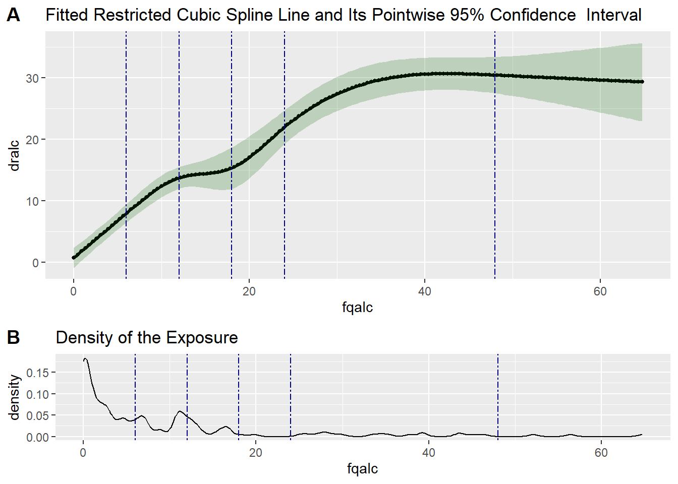
Exercise: Testing the Linearity of the Measurement Error Model for Total Calories in VS
# Test if the calibration model is linear
test5 <- testLinear(ds = valid_data,
outcome = "drcal",
var = "fqcal",
adj = c("fqtfat", "fqalc", "agec"),
nknots = 5,
method = "lm",
densplot = TRUE)
test5$testOfLinearity
LRT-based chisq df
Test of non-linear cubic spline terms 1.728298 3
Test of overall curvature (i.e. all cubic spline terms) 9.480342 4
Test of linear term only. 7.752044 1
p value
Test of non-linear cubic spline terms 0.6307
Test of overall curvature (i.e. all cubic spline terms) 0.0502
Test of linear term only. 0.0054# Plot spline
test5$fittedCBSplineCurve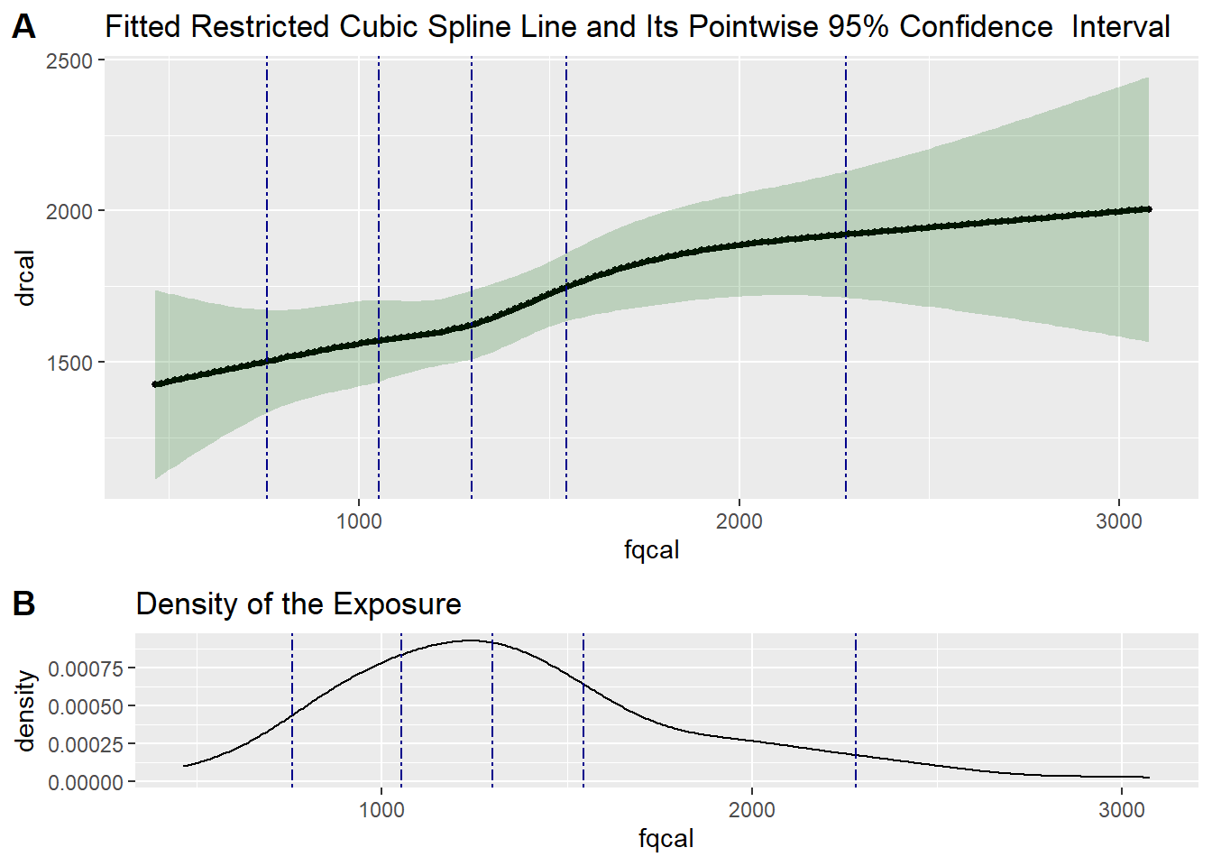
Exercise: Linearity of the Measurement Error Model for Total Fat in the VS
# Test if the calibration model is linear
test4 <- testLinear(ds = valid_data,
outcome = "drtfat",
var = "fqtfat",
adj = c("fqcal", "fqalc", "agec"),
nknots = 5,
method = "lm",
densplot = TRUE)
test4$testOfLinearity
LRT-based chisq df
Test of non-linear cubic spline terms 1.989486 3
Test of overall curvature (i.e. all cubic spline terms) 9.879113 4
Test of linear term only. 7.889627 1
p value
Test of non-linear cubic spline terms 0.5746
Test of overall curvature (i.e. all cubic spline terms) 0.0425
Test of linear term only. 0.0050# Plot spline
test4$fittedCBSplineCurve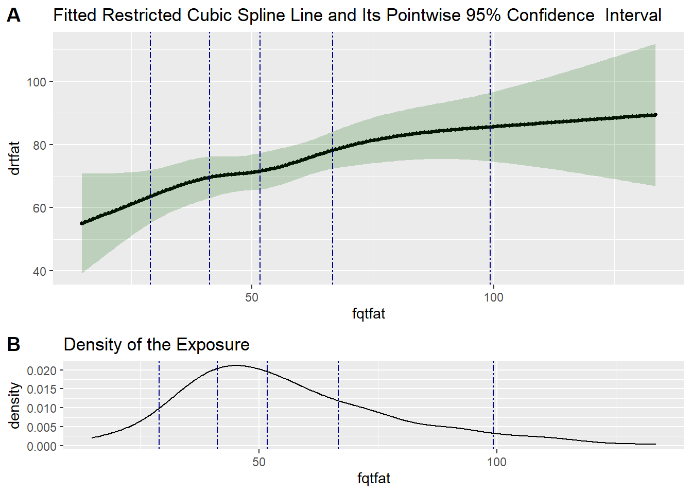
2. Reliability Study Available
The R package RegCalReliab addresses measurement error in covariates when either an internal or an external reliability study is available. More details of the usage of the package are here.
3. Other Packages on Regression Calibration
The R package mecor implements regression calibration for linear model with continuous outcomes. More details of the usage of the package can be find here.